How to Optimize Your 4-Lay… | PCBA & EMS Insights

Why a Bad 4-Layer Stackup Can Derail Both Signal Integrity and Production Schedules

A PCB stackup is more than a mechanical arrangement of copper and dielectric. It’s the electromagnetic skeleton that determines whether a high‑speed signal reaches its destination intact or radiates enough energy to fail compliance testing. In a 4‑layer board, every layer assignment either helps the signal find a low‑inductance return path or forces it to wander through a maze of vias and split planes. When the stackup is wrong, the symptoms are immediate: impedance mismatches that turn clean digital edges into ringing nightmares, crosstalk that corrupts sensitive analog channels, and electromagnetic interference that can push a product out of EMC limits by 10 dB or more.

These aren’t just simulation curiosities. An inadequately designed stackup can precipitate a cascade of real‑world failures — electromagnetic interference (EMI), signal crosstalk, and impedance mismatches — that force layout re‑spins and delay production schedules. Engineers who treat the 4‑layer stackup as an afterthought often discover that a few extra days of careful optimization at the design stage would have saved weeks of debug and thousands of dollars in rushed prototype turns. When a board enters volume manufacturing with marginal impedance control, yield and reliability both suffer, turning what looked like a cost‑saving measure into an expensive lesson.

The good news is that optimizing a 4‑layer stackup for signal integrity isn’t a black art. It’s a series of deliberate choices about layer sequencing, dielectric thickness, copper weight, and material properties — choices that can be validated with the shop floor data your fabricator already has. The following sections lay out the physics, the cost trade‑offs, and the step‑by‑step workflow that removes guesswork from controlled impedance, so the stackup you sign off on actually behaves the way you expect.

How the Classic Signal‑Ground‑Power‑Signal (SGPS) Stackup Delivers Controlled 50 Ω Impedance

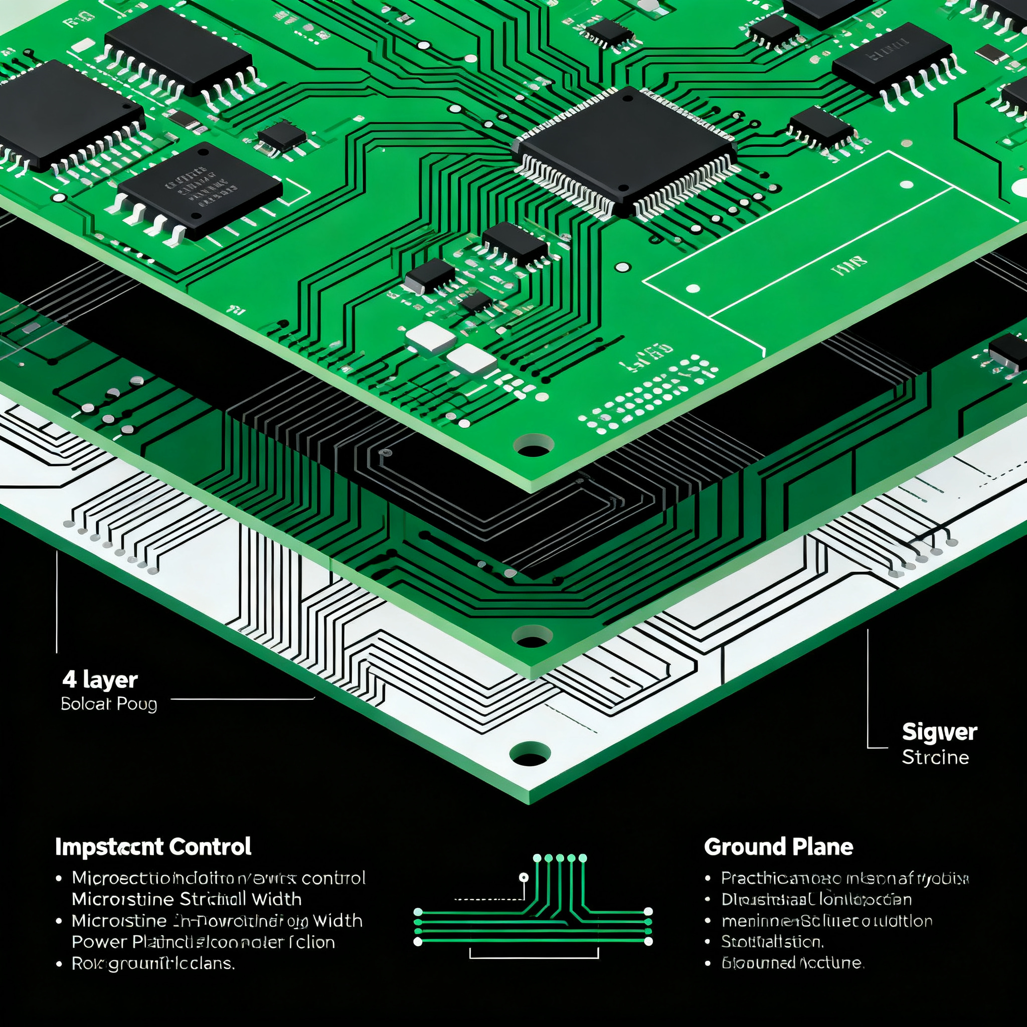
The most widely adopted 4‑layer stackup places signals on the outer layers (L1 and L4) and planes on the inner layers — ground on L2 and power on L3. This arrangement, designated Signal‑Ground‑Power‑Signal (SGPS), works because it puts a continuous reference plane immediately adjacent to every routing layer. The ground plane is typically placed on Layer 2, directly beneath the top signal layer, to provide a low‑impedance return path for signals. That proximity — often just 3–6 mils of prepreg — creates tight capacitive coupling, which reduces loop inductance and constrains the return current precisely under the forward trace. The result is clean, predictable transmission‑line behavior that lets you hit 50 Ω single‑ended impedance with standard trace widths.

The physics that makes SGPS reliable also makes it forgiving. This tight coupling helps in maintaining controlled impedance, typically targeting 50 ohms for critical high‑speed traces, thereby preserving signal integrity. Likewise, inner planes give better reference for high‑speed signals, cleaner return paths, and a built‑in path for power distribution. An alternative configuration — SPGS, where the power plane occupies L2 and ground moves to L3 — can be useful in certain mixed‑signal scenarios but sacrifices the best possible return path on the primary routing layer. The table below compares these two sequences with typical 1.6 mm FR4 constructions.

Parameter	SGPS (L1‑Signal, L2‑GND, L3‑PWR, L4‑Signal)	SPGS (L1‑Signal, L2‑PWR, L3‑GND, L4‑Signal)	Unit / Notes
Typical core thickness between L2–L3	0.71 mm (28 mil)	0.71 mm (28 mil)	FR4, 1.6 mm total thickness
Prepreg thickness L1–L2 (H1)	0.20 mm (7.9 mil)	0.20 mm (7.9 mil)	Contact fabricator for exact value
Prepreg thickness L3–L4 (H3)	0.20 mm (7.9 mil)	0.20 mm (7.9 mil)	Symmetrical construction preferred
Primary return path on top layer	Solid GND plane, lowest loop inductance	Power plane; may be segmented, raising inductance	Critical for edge rates > 1 ns
Calculated 50 Ω single‑ended trace width (1 oz Cu, Dk=4.3)	~8.0 mil	~8.5–9.0 mil (depends on plane contiguity)	SGPS yields more consistent impedance
EMI performance (far‑field radiation)	Excellent — tightly coupled return path	Good, but higher risk if power plane splits	SGPS preferred for FCC/CE compliance
Power‑plane decoupling efficiency	Adjacent to ground plane on L3, good high‑frequency decoupling	Power plane on L2 reduces via inductance for top‑side ICs	Trade‑off; SGPS usually wins for signal integrity
Recommended for high‑speed digital	Yes — standard choice	No — only when specific IC power pin access demands it

SGPS works because it creates a well‑defined, symmetric transmission‑line environment on both outer layers. The ground plane on L2 serves as the primary reference for all L1 signals; the power plane on L3, when coupled to ground through the thin core dielectric, behaves as an AC ground for L4 signals. This dual‑reference approach is what makes a 50 Ω design repeatable from lot to lot, as long as the dielectric materials are consistent. SPGS can provide superior capacitive coupling between power and ground planes because they are separated by a thinner prepreg in some constructions, but that benefit rarely outweighs the signal‑integrity penalty of referencing high‑speed traces to a potentially slotted power plane. Unless your design explicitly needs the power plane on L2 to minimize pin‑side via inductance for a large BGA on the top side, SGPS is the safer default.

Standard Fabricator Stackups vs. Custom One‑Offs: The Real Cost and Lead‑Time Trade‑Off

Every PCB shop maintains a set of standard laminate constructions that it procures in volume. These “factory‑preferred” stackups define the core and prepreg materials, copper weights, and pressed thicknesses that will go through the lamination press without special setup. When you design to one of these standards, you’re effectively buying a known impedance solution that thousands of boards have already validated. When you deviate — specifying a thicker dielectric to hit a particular differential impedance, or switching to a Rogers 4350B core for lower loss — you trigger a custom stackup that forces the fabricator to stock a new material combination, run a dedicated press cycle, and build out‑of‑profile test coupons.

The difference in time and money is more than trivial. Using standard dielectric builds dramatically reduces lead time and cost variability. According to fabrication data from AtlasPCB, using your manufacturer’s standard stackup saves 15–25% versus custom builds and reduces lead time by 2–3 days. For a prototype run that’s already schedule‑critical, those three days can be the difference between making the integration deadline and missing it.

That doesn’t mean custom stackups are never justified. Higher frequency designs (above 1 GHz) benefit from low‑loss materials like Rogers, which offer a lower Dk (3.0–3.5) and superior signal integrity. When loss budgets are tight or you’re designing a microwave front‑end on a 4‑layer board, a custom construction with a controlled‑Dk substrate becomes essential. But for the vast majority of digital boards running at a few hundred megahertz, the standard FR4 SGPS stackup is not only adequate — it’s the fastest and most economical way to achieve consistent 50 Ω impedance.

Comparison Metric	Standard Fabricator Stackup (FR4, SGPS)	Custom Low‑Loss Stackup (e.g., Rogers/FR4 hybrid)	Selection Criteria & Failure Boundary
Typical prototype lead time	5–7 days	8–11 days	Added 2–3 days for custom (AtlasPCB)
Cost adder vs. standard 4‑layer	Baseline	+15–25%	Applies to both small and medium volumes
Dk tolerance	±0.2 (typical FR4)	±0.05 (Rogers 4350B)	Critical for impedance repeatability above 1 GHz
Loss tangent @ 1 GHz	0.020	0.0037	Lower loss means less jitter on long traces
50 Ω trace width (microstrip, 1 oz Cu)	~8.0 mil on standard 7.9 mil prepreg	~7.5 mil on 8 mil Rogers prepreg (Dk=3.48)	Custom stackup can yield slightly narrower traces
Impedance coupon verification	Manufacturer may already have coupon data for standard construction	Requires new coupon design; additional TDR cost	First‑article cost climbs further
When to choose	Digital/analog < 500 MHz, general embedded systems	RF front‑ends, multi‑gigabit serial links, long backplane traces	Triggered by insertion‑loss budget or phase‑stability requirements

The key takeaway is that a standard stackup is not a compromise — it’s an optimized solution that leverages the fabricator’s volume materials. By aligning your design with these pre‑qualified constructions, you get a known impedance outcome while keeping procurement simple. When simulations show that a standard FR4 build cannot meet your insertion‑loss target at the Nyquist frequency of your serial link, that’s the time to engage your fabricator early, share the link budget, and co‑design a custom stackup that hits the required impedance and loss simultaneously.

From Impedance Calculator to First‑Article Verification: A Step‑by‑Step Workflow Designers Can Trust

Getting to a reliable 50 Ω value isn’t about picking a trace width from a textbook table. It’s a closed‑loop process that begins with the manufacturer’s real material data and ends with a time‑domain reflectometer (TDR) measurement on the first‑article board. Instead of selecting a generic trace width, obtain the fabricator’s actual stackup, including finished copper thickness, dielectric thickness, and material properties. Every shop has slightly different laminate sources and press cycles; a 0.20 mm prepreg from one supplier may compress to 0.18 mm after lamination. Using the actual cured thicknesses — not the nominal pre‑preg numbers — is what makes the impedance calculation meaningful.

Once you have that data, the engineering steps are straightforward, but skipping any one of them turns controlled impedance into an uncontrolled variable. The workflow below distills years of field experience into a sequence that avoids the most common mistakes, such as routing high‑speed traces over split power planes or ignoring the effect of copper‑pour density on dielectric constant. Proper layer sequencing minimizes crosstalk and enhances signal integrity, but only if the trace geometry is calculated against the right dielectric stack.

Step	Action	Critical Checkpoint
1. Request fabricator stackup data	Ask for the exact core/prepreg part numbers, pressed thicknesses, copper weights (after plating), and Dk/Df values at your test frequency (e.g., 1 GHz).	Confirm the data is from production‑proven builds, not datasheet nominal.
2. Model transmission line in a field‑solver	Use Polar Instruments Si8000, Saturn PCB Toolkit, or HyperLynx to compute the trace width for 50 Ω single‑ended (microstrip on L1/L4). Model as a coated microstrip if solder mask is present; its Dk (~3.5–4.0) can shift impedance by 1–2 Ω.	Correlate width with fabricator’s minimum etch capability.
3. Assign a solid reference plane	Route all critical 50 Ω traces over continuous ground (SGPS). Never route over a split in the power plane; if unavoidable, bridge the gap with stitching capacitors on either side of the split.	Check with post‑layout simulation or visual inspection.
4. Design an impedance test coupon	Include a coupon with 4‑inch traces of the calculated width on a dedicated test area of the panel, matching the layer stack. Specify TDR testing at the manufacturing stage.	Coupon must use the same copper thickness and plane spacing as the production board.
5. First‑article TDR verification	After fabrication, have the manufacturer measure the coupon’s impedance and provide a TDR plot. Accept 50 Ω ±10% for most digital designs; tighten to ±5% for sensitive serial links.	If out of tolerance, iterate with material or line‑width adjustments.

Tip: A common trap is designing for 50 Ω on a layer referenced to a power plane that’s heavily perforated by anti‑pads under a dense BGA. The effective Dk drops locally, and the trace impedance can spike. The safest approach is to always reference high‑speed signals to a solid ground plane. If you must use the power plane as a reference, ensure uninterrupted copper beneath the entire trace length, and use decoupling capacitors to stitch the power plane to ground at both ends of the signal path.

This workflow doesn’t add significant engineering time when you integrate it from the start of layout. The fabricator data request takes one email, and the field‑solver calculation takes minutes. The real cost is debugging an uncontrolled impedance board after it’s built — a task that can consume days and often leads to an emergency re‑spin with the very stackup data you should have requested at the beginning.

For teams producing a few hundred or a few thousand units, partnering with an assembly provider that understands controlled‑impedance requirements can close the loop. NovaPCBA’s assembly services handle 4‑layer controlled‑impedance boards daily, with incoming inspection that verifies impedance coupons before a single component is placed, so what you simulated is what you get on the production floor.

4‑Layer Stackup Q&A: When to Leave 2 Layers Behind, Choosing SGPS or SPGS, and FR4 Myths

The following questions reflect the conversations engineers and procurement leads have when a 4‑layer board first appears in a project BOM. They go beyond textbook definitions to address the real‑world trade‑offs that influence schedule, cost, and signal integrity.

Q: When should I move from a 2‑layer to a 4‑layer PCB?
Use a 4‑layer PCB when routing density, signal integrity, grounding, EMI control, or power distribution makes a two‑layer design difficult to manage reliably. A 2‑layer board forces return currents to travel through arbitrary ground‑fill shapes, creating large loop areas that radiate. A 4‑layer board adds dedicated inner planes that provide low‑inductance return paths and enable controlled impedance for high‑speed traces. If you find yourself stitching ground on a 2‑layer board with dozens of vias, or if your board fails radiated emissions on the first pass, the cost of adding two inner planes is almost always lower than the cost of debug and re‑spin.

Q: Which 4‑layer stackup is best for most designs — SGPS or SPGS?
The SGPS (Signal‑Ground‑Power‑Signal) arrangement is the most widely used because it places the ground plane directly under the top signal layer, delivering the lowest loop inductance and best EMI performance. An alternative, though less common, configuration is the SPGS stackup, where the power plane occupies Layer 2 and the ground plane is on Layer 3. SPGS can reduce via inductance to power pins on the top side, but at the expense of referencing high‑speed signals to a plane that may be split or slotted. SGPS is the safer default unless your specific IC pinout absolutely demands the power plane on L2.

Q: Do I need expensive low‑loss materials for a 4‑layer board running at a few hundred MHz?
Not necessarily. Standard FR4 with a dielectric constant in the range of 4.2–4.5 works well below 1 GHz when the stackup is properly designed. While standard PCB FR4 material (Dk typically 4.2–4.5) is common, higher frequency designs (above 1 GHz) benefit from low‑loss materials like Rogers. For designs above 1 GHz or with very long, loss‑sensitive traces, migrating to a low‑Dk substrate can improve signal integrity, but that step is normally triggered by a failing link budget, not by clock frequency alone.

Q: How do I guarantee 50 Ω single‑ended impedance without going back and forth with the fabricator?
Start with the fabricator’s actual stackup data — finished copper thickness, dielectric heights after pressing, and material Dk/Df at your test frequency — before calculating trace geometry. Use a field‑solver like Polar or Saturn PCB Toolkit to compute the required width. Then ask the manufacturer to confirm the result with an impedance test coupon on the first‑article board. If you provide the stackup and the calculated width in your fabrication drawing, and the shop verifies the coupon before shipping, the impedance becomes a locked‑in parameter rather than a negotiation.

Q: Can I mix high‑speed and sensitive analog traces on the same 4‑layer board?
Yes, but keep them well separated and avoid routing analog traces directly over split power planes. Use the continuous ground plane as the primary reference for both domains. Guard traces can help, but they must be tied to ground with a via stitch density that prevents them from becoming radiating antennas. Before adding moats or isolation slots, simulate the return‑current path; an improperly placed moat can force return currents around a slot, increasing loop area and coupling noise into other circuits.

Q: What’s the true lead‑time and cost penalty of a custom 4‑layer stackup versus a standard one?
A custom stackup typically adds 2–3 days to prototype lead times and increases cost by 15–25% compared to a fabricator’s standard dielectric builds, as reported by multiple board shops. Unless your impedance or high‑frequency loss requirements cannot be met with a standard FR4 SGPS construction — for example, when you need a Dk of 3.3 to hit a 100 Ω differential impedance with trace‑width constraints — adopting the manufacturer’s standard stackup is the faster, more economical path.

Takeaway: The majority of successful 4‑layer designs achieve signal‑integrity goals with a well‑executed SGPS stackup on standard FR4. The real skill lies not in exotic materials but in closing the impedance‑control loop early with the fabricator’s actual data, verifying the result on a test coupon, and respecting the return‑path integrity that the stackup provides. When those fundamentals are in place, a 4‑layer board can handle high‑speed interfaces, sensitive analog, and dense power distribution without demanding a custom laminate solution.

For teams moving from prototype to production, NovaPCBA’s assembly capabilities cover the full spectrum of controlled‑impedance 4‑layer boards, with incoming material verification that ensures the stackup you validated is the one that hits the pick‑and‑place line — keeping your 50 Ω traces right where you calibrated them.

How to Optimize Your 4-Layer PCB Stackup for Signal Integrity: Real-World Impedance Control Examples